flowchart LR
    X((X)) --> Y((Y))
    W((W)) --> Y
    XW((X times W)) --> Y
    X -. "moderated by W" .- W
    classDef default fill:#2e4057,color:#ffffff,stroke:#ff9933,stroke-width:3px,rx:10px,ry:10px;
18 Moderation Analysis
18.1 Moderation in Context
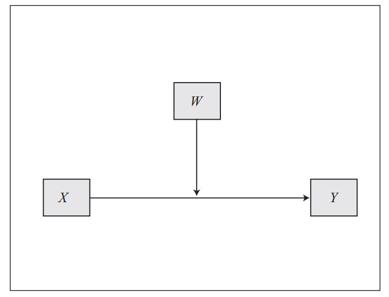
Chapter 17 asked how X reaches Y. Moderation asks a different question: when or for whom does X reach Y at all? A price discount may raise sales, but only for price-sensitive segments. A training course may raise performance, but only for new hires. The variable that changes the strength (or direction) of the X-to-Y relationship is called a moderator (Aiken and West 1991).
NoteWhat a moderator is and is not
A moderator changes the slope of X on Y. It is not a mediator (Chapter 17), which explains the mechanism, and it is not a confounder, which biases the estimate of X on Y. The defining feature is that the effect of X depends on the value of the moderator.
TipWhy boundary conditions matter
A bottom-line lift that is real on average but absent in a large segment is a lift that can be targeted more efficiently. Moderation analysis locates the segments where the effect lives, so the intervention can be priced and placed accordingly.
TipWhat moderation surfaces
| Question moderation answers | Example | Standard visual |
|---|---|---|
| Does the effect differ across groups? | Price elasticity by region | Small-multiples regression by group |
| Does the effect differ across conditions? | Promotion lift inside vs outside campaign weeks | Faceted scatter with regression line |
| Does the effect differ across time? | Channel-attribution stability across years | Coefficient over time with confidence band |
| Does the effect differ across levels of a continuous moderator? | Discount effect moderated by income | Simple-slopes plot at low, mean, high |
18.2 The Moderation Model
Moderation is implemented as an interaction term. The linear model becomes Y = b0 + b1 X + b2 W + b3 X W + e. The b3 coefficient on the product X W is the moderation effect: the amount by which the slope of X on Y shifts per unit of W (Cohen, Cohen, West and Aiken 2003).
WarningThe main effects change meaning when an interaction is present
With X W in the model, b1 is no longer the average slope of X on Y. It is the slope of X when W equals zero. Whether zero is a meaningful value of W is the question centering is meant to answer.
18.3 Fitting an Interaction with lm
The x * w shorthand in R expands to the main effects plus the interaction. The summary prints three coefficients of interest: the conditional slope of X at W equals zero, the conditional slope of W at X equals zero, and the interaction b3.
NoteReading the interaction row
The price:income row is b3: a positive value means the price slope gets steeper as income rises, a negative value means it flattens. The size of b3 is the change in the price slope per one-unit rise in income.
18.4 Centering Predictors
Centering each predictor on its mean makes zero a meaningful reference point and turns b1 and b2 into average slopes at the mean of the other predictor. The interaction coefficient b3 is invariant to centering; only the main effects change.
TipThe interaction is stable, the main effects are not
Notice that the price:income and price:income_c rows print the same coefficient. What changes between the raw and centred fits is the price main effect, because the reference value of the moderator changed from zero to the sample mean.
18.5 Simple Slopes
The effect of X on Y at a specific value of W is called a simple slope. The standard probing scheme (Aiken and West 1991) evaluates the simple slope at the mean and at one standard deviation below and above the mean of W.
NoteWhat the three numbers tell you
A steeper positive slope at high income than at low income confirms a synergistic interaction. A sign change between low and high income would be a crossover interaction, where the direction of the X to Y effect flips across the moderator’s range.
18.6 Visualising Moderation
The standard picture of a moderated effect is three regression lines: the slope of Y on X at low, medium, and high values of W. A crossing or fanning pattern tells the story at a glance.
TipShape before significance
Fans that open to the right, fans that close, and lines that cross are all substantively different stories. The picture should guide the interpretation; the numerical probing confirms it.
18.7 Categorical Moderator
When W is a factor, the interaction splits the slope of X across its levels. R’s lm handles this automatically with dummy coding; the interaction rows compare each non-reference level’s slope against the reference.
NoteReading dummy interaction rows
The price row is the slope inside the reference level (alphabetically first, Online here). Each price:segmentXxx row is the difference between that level’s slope and the reference slope. Summing the two gives the group-specific slope.
18.8 Johnson-Neyman Region of Significance
Simple slopes at three cherry-picked values of W answer the question at three points; the Johnson-Neyman (1936) technique answers it across the entire range of W by plotting the conditional slope and its 95 percent confidence band, then reading off the values of W at which the band excludes zero.
WarningWhere the band crosses zero is the decision boundary
Income values where the confidence band is entirely above (or below) zero are the region where the price effect is reliably different from zero. Values where the band straddles zero are the region where the data are not sharp enough to commit.
18.9 Moderation in Logistic Regression
Moderation in a glm works exactly as in lm, but the interaction coefficient is on the log-odds scale. Exponentiating an interaction term gives the ratio of odds ratios, which tells the reader how much the effect of X on the odds of Y changes per unit of W.
TipInteraction on the log-odds scale
An interaction odds ratio above 1 says the tenure effect makes churn more likely for the non-reference tier relative to the reference. Below 1 says the opposite. The sign of b3 on the log-odds scale and the odds-ratio direction always agree.
18.10 Effect Size for an Interaction
The practical size of a moderation effect is the share of additional variance the interaction adds once the main effects are in the model. This is read off a nested-model comparison as the change in R-squared (or, on a GLM, the change in deviance).
NoteTwo complementary numbers
Delta R-squared puts the interaction’s contribution on a zero-to-one scale. The F test from anova asks whether that contribution is larger than sampling noise would produce. Reporting both keeps the practical and statistical pictures separate.
18.11 Moderation versus Mediation
The two frameworks sound similar and are easy to confuse. They answer different questions, use different models, and are rarely interchangeable.
TipQuick contrast
Mediation (Chapter 17) asks through what mechanism X reaches Y and introduces a mediator M on the path X to M to Y. Moderation asks under what condition the effect of X on Y holds and introduces a moderator W that enters as an interaction X times W. A single study can have both: a moderated mediation has an indirect effect whose size depends on W. Hayes (2017) gives the integrated framework.
WarningWhich variable is on which role is a design decision
Whether a variable should be treated as a mediator or a moderator depends on the theoretical claim, not the data. The same third variable can take either role in different studies; the choice is made before fitting the model, not after.
18.12 Moderation versus Interaction
Moderation and interaction share the same regression machinery — both add an X*W product term — but they answer different conceptual questions and warrant different framings in the report.
TipThe framing distinction
Moderation is asymmetric: X is the focal predictor, and W modifies the strength (or sign) of X’s effect on Y. Interaction is symmetric: X and W are co-equal predictors that jointly determine Y, with neither privileged. The same b3 coefficient supports either reading; the choice depends on the theoretical claim being made and on which framing makes the chart legible to the audience.
WarningWhere additive thinking fails
A market that is high on price-sensitivity and low on awareness will not respond to a discount the same way as one that is high on both, even when an additive model assigns them the same total exposure. This is where the interaction frame outperforms the moderation frame: when neither variable has natural priority and the joint pattern is the substantive story. The visual signature is a contour plot or a small-multiples grid, not a three-line simple-slopes plot.
18.13 Reporting a Moderation Analysis
A moderation report reuses the six-section skeleton of Chapters 11 to 17 and adds a probing section.
TipSix-section moderation report
- Question and hypothesised boundary condition (X, W, and the proposed form of interaction), (2) sample and measurement, (3) fit table with centred predictors and the interaction coefficient, (4) probing: simple slopes at low, mean, high values of W plus the Johnson-Neyman plot, (5) effect size: Delta R-squared and the nested-model F, (6) business decision and the segment where the effect lives. Keeping the skeleton aligned with the Chapter 11 to 17 reports makes descriptive, inferential, predictive, mechanistic, and boundary-condition studies directly comparable.
Summary
| Concept | Description |
|---|---|
| Concept | |
| What Moderation Is | A moderator changes the strength or direction of an effect |
| Boundary Conditions | When and for whom an effect holds |
| Modelling and Interpretation | |
| Moderation Model | Y ~ X + Z + X:Z — interaction term carries the moderation |
| Centering Predictors | Center continuous predictors so main effects stay interpretable |
| Reading Interaction Row | Significance and sign of the interaction coefficient |
| Simple Slopes | Effect of X at low, mean, and high levels of Z |
| Visualising Moderation | Plot lines of X-on-Y at different Z values |
| Shape Before Significance | Inspect the plot before reading the significance test |